Since all data processing in the Zantiks units is performed live, it is necessary to outline which data you would like to be processed and how this data will be exported in zanscript.
This page will explain how to use the LOGCREATE, LOGDATA and LOGRUN commands in a script to organise zone data output in two different formats (this is not exclusive, you may export your data in any format that you wish). Here we provide an example of exporting all zone data on a single line per data point for a thigmotaxis assay in the MWP system; plus an example of exporting zones data across multiple lines per data point for a scototaxis assay in the AD system.
For more detailed explanations about processing and exporting data using LOGCREATE, LOGDATA and LOGRUN commands, you can refer to the support pages on Writing and exporting data and Measuring distance and zone use.
Explanations for the syntax, LOGCREATE, LOGAPPEND and LOGRUN can be found in the Zanscript syntax manual.
NOTE: The command LOGRUN() will tell the unit to output the last line of data as detailed in the previous LOGCREATE command, so if there are two LOGRUN() commands the previous LOGCREATE command will be output twice in the data file.
Script Explanation, single line of data output
Before running this experiment, the appropriate assets need to be loaded into the Asset Directory. You will need 2 bitmap (.bmp) files: one defines arenas and another defines zones. You may define as many zones within your experiment as you choose. The order of the zones will also be specified by the .bmp file. Some general information about the ordering of arenas and zones can be found here. If you are unsure about the order in which your zones are represented in the .bmp asset file, please get in touch.
See the Calibrating your Zantiks unit page and Asset building in the MWP unit page for details on how to create assets for the Zantiks MWP system.
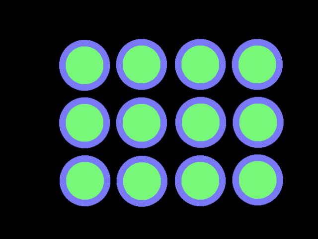
The script below demonstrates how to export zones data for a thigmotaxis experiment in a 12-well plate for zebrafish larvae. Multiple endpoints can be processed and exported for zones data, including distance travelled in zone, time spent in zone and number of entries into zone.
DEFINE BIN 1
DEFINE NUM_SAMPLES 10

SET(TARGET_SIZE,2)
SET(DETECTOR_THRESHOLD,6)

SET(AUTOREF_MODE,MOVEMENT)
SET(AUTOREF_TIMEOUT,60)

SET(COUNTER1,COUNTER_ZERO)
The above lines of code DEFINE timings used later in the script and the settings required for tracking.
ACTION MAIN

 LOAD(ARENAS,"a12.bmp")
 LOAD(DETECTORS, "z12dz.bmp")

 LOGCREATE("TEXT:RUNTIME|TEXT:TEMPERATURE|TEXT:CONDITION|TEXT:TIME_BIN")

 LOGAPPEND("TEXT:D.A1.Z1|TEXT:D.A1.Z2|TEXT:D.A2.Z1|TEXT:D.A2.Z2|TEXT:D.A3.Z1|TEXT:D.A3.Z2|TEXT:D.A4.Z1|TEXT:D.A4.Z2")
 LOGAPPEND("TEXT:D.B1.Z1|TEXT:D.B1.Z2|TEXT:D.B2.Z1|TEXT:D.B2.Z2|TEXT:D.B3.Z1|TEXT:D.B3.Z2|TEXT:D.B4.Z1|TEXT:D.B4.Z2")
 LOGAPPEND("TEXT:D.C1.Z1|TEXT:D.C1.Z2|TEXT:D.C2.Z1|TEXT:D.C2.Z2|TEXT:D.C3.Z1|TEXT:D.C3.Z2|TEXT:D.C4.Z1|TEXT:D.C4.Z2")
 LOGAPPEND("TEXT:C.A1.Z1|TEXT:C.A1.Z2|TEXT:C.A2.Z1|TEXT:C.A2.Z2|TEXT:C.A3.Z1|TEXT:C.A3.Z2|TEXT:C.A4.Z1|TEXT:C.A4.Z2")
 LOGAPPEND("TEXT:C.B1.Z1|TEXT:C.B1.Z2|TEXT:C.B2.Z1|TEXT:C.B2.Z2|TEXT:C.B3.Z1|TEXT:C.B3.Z2|TEXT:C.B4.Z1|TEXT:C.B4.Z2")
 LOGAPPEND("TEXT:C.C1.Z1|TEXT:C.C1.Z2|TEXT:C.C2.Z1|TEXT:C.C2.Z2|TEXT:C.C3.Z1|TEXT:C.C3.Z2|TEXT:C.C4.Z1|TEXT:C.C4.Z2")
 LOGAPPEND("TEXT:T.A1.Z1|TEXT:T.A1.Z2|TEXT:T.A2.Z1|TEXT:T.A2.Z2|TEXT:T.A3.Z1|TEXT:T.A3.Z2|TEXT:T.A4.Z1|TEXT:T.A4.Z2")
 LOGAPPEND("TEXT:T.B1.Z1|TEXT:T.B1.Z2|TEXT:T.B2.Z1|TEXT:T.B2.Z2|TEXT:T.B3.Z1|TEXT:T.B3.Z2|TEXT:T.B4.Z1|TEXT:T.B4.Z2")
 LOGAPPEND("TEXT:T.C1.Z1|TEXT:T.C1.Z2|TEXT:T.C2.Z1|TEXT:T.C2.Z2|TEXT:T.C3.Z1|TEXT:T.C3.Z2|TEXT:T.C4.Z1|TEXT:T.C4.Z2")

 LOGRUN()

 AUTOREFERENCE()

 INVOKE (SAMPLE, NUM_SAMPLES)

COMPLETE
The ACTION MAIN is the whole experiment outline. The actions listed here are further explained below:
- LOAD(ARENAS,"a12.bmp"): loads a bitmap file called a12.bmp from the Assets Directory. In this example, a .bmp which outlines the arenas for a 12-well plate is loaded.
- LOAD(DETECTORS,"z12dz.bmp"): loads a bitmap file called z12dz.bmp in the Assets Directory which outlines the size and shape of the zones per arena.
- LOGCREATE, LOGAPPEND and LOGRUN(): write the headings for the data output in the order in which the processed data will be reported (this is specified by the .bmp file).
- LOGCREATE: specifies a beginning of a line of data which comprises TEXT: cells. Any characters following TEXT: are written onto the data file. For example, TEXT:RUNTIME| will write the word "RUNTIME" into the first cell on the .csv file.
- LOGAPPEND: allows a continuation of the LOGCREATE command when there is a large amount of data to be written. It will continue on the same row within the .csv file.
- LOGRUN: tells the unit to output the data at this point in the script on the .csv data file as specified in the previous LOGCREATE line of code.
- For more detailed information on these commands see the Writing and exporting data support page.
- The system will then take an autoreference for tracking and INVOKE the action called SAMPLE which is detailed later in the script and repeats this action a number of times as DEFINED at the top of the script by NUM_SAMPLES.
- COMPLETE: signals the system that the ACTION MAIN is complete. Every ACTION must end with a COMPLETE.
- In the example above D. = distance travelled in zone data, C. = count/number of entries into zone data, T. = time spent in zone data.
ACTION SAMPLE

 SET(COUNTER1,COUNTER_INC)

 LOGDATA(DATA_SNAPSHOT,"begin")
 WAIT(BIN)
 LOGDATA(DATA_SNAPSHOT,"end")
 LOGDATA(DATA_SELECT,"begin")
 LOGDATA(DATA_DELTA,"end")

 LOGCREATE("RUNTIME|TEMPERATURE1|TEXT:BRIGHT|COUNTER1")
 LOGAPPEND("ZONE_DISTANCES:A1-12 Z1-2|ZONE_COUNTERS:A1-12 Z1-2|ZONE_TIMERS:A1-12 Z1-2")
 LOGRUN()

COMPLETE
The action SAMPLE processes data in 1 second time bins for multiple parameters:
- The counter labelled COUNTER 1 is set to count incrementally.
- LOGDATA(DATA_SNAPSHOT, "begin"): logs the tracking data of the organism and calls this data "begin". The system then WAITs for a period of time in seconds DEFINED as BIN at the top of the script.
- LOGDATA(DATA_SNAPSHOT, "end"): makes another log of the tracking data after the TIME_BIN and calls this data "end".
- The following LOGDATA commands (DATA_SELECT,"begin") and (DATA_SELECT,"end") instructs the unit to calculate the difference between "begin" and "end".
- The final series of LOGCREATE, LOGAPPEND and LOGRUN() commands specify the content for a row of data and outputs it into the .csv file. In this case:
- The time the data is collected during the experiment is written using the command RUNTIME.
- Followed by the system temperature of the time the data was collected.
- The phase the experiment was in. In this example, the phase was labelled BRIGHT.
- COUNTER1 will input the time bin
- ZONE_DISTANCES asks the system to calculate the distance travelled for all arenas and zones
- ZONE_COUNTERS outputs the number of entries into each zone (Entries is the default methods. See Target Zone Methods page for more information on the different ways to use ZONE_COUNTERS.)
- ZONE_TIME outputs the amount of time spent in each zone
- A1-12 Z1-2 asks for this data to be output for arenas 1-12 and zones 1-2 which are specified by the .bmp file
Script Download, single line
To download the exporting_zone_data_demo_MWP demo script as a .zs file (file type Zantiks software reads), choose the Save File As option in the right-click dialogue box. Clicking on the script name hyperlink will open a read-only version of the script.
Script download: exporting_zone_data_MWP.zs
Assets
You will need to upload the asset into the Asset directory on your Zantiks Control Console and ensure the correct asset name is in the LOAD(ZONES,"name_of_asset") command in the script.
See the Calibrating your Zantiks unit page and Asset building in the MWP unit page for details on how to create assets customised to your system.
Script Explanation, multiple lines
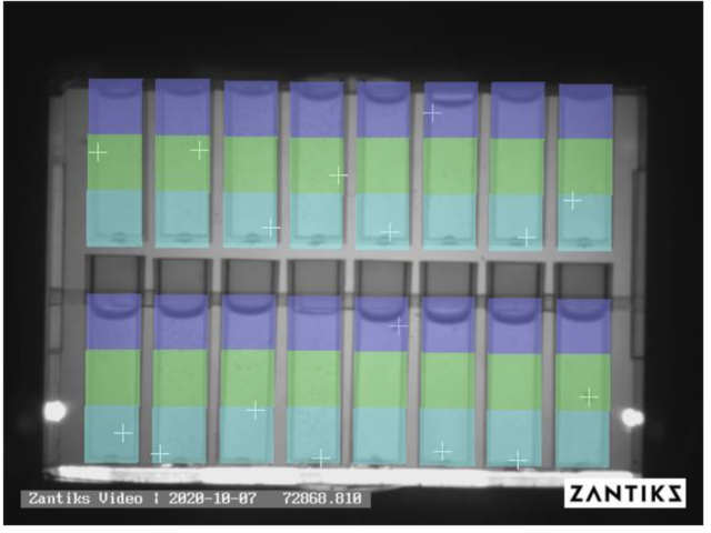
This tutorial, is presented in two part videos. The videos demonstrate how to obtain processed results from your experiments in a Zantiks AD unit. The data file will include distance travelled in arenas, in different zones; time spent in different zones; and the number of times different zones are entered.
In this example we have used a sample scototaxis script in the AD unit, which illuminates half of the chamber from the built-in screen below the tank. The chamber is set up with two arenas, for two singly housed animals, and each arena has two zones.
Part 1: Runs through how to use the LOGDATA, LOGCREATE and LOGRUN functions in your script.
Part 2: illustrates the use of LOGDATA, LOGCREATE, LOGAPPEND and LOGRUN, going through a section of the script, in this case called ACTION WRITEDATA, which is used to output the data at different stages during the experiment. It also shows how the results data, downloaded in a .csv file, can be displayed in a spreadsheet.
Script Download, multiple lines
To download the scototaxis_demo_AD script as a .zs file (file type Zantiks software reads), choose the Save File As option in the right-click dialogue box. Clicking on the script name hyperlink will open a read-only version of the script.
Script download: scototaxis_demo_AD.zs
Assets
You will need to upload the asset into the Asset directory on your Zantiks Control Console and ensure the correct asset name is in the LOAD(ZONES,"name_of_asset") command in the script.
See the Calibrating your Zantiks unit page and Asset building in the AD unit page or Asset building in the LT unit page for details on how to create assets customised to your system.


%3F)